Quick Start for tomo_display

If you are running the licensed version of IDL then start IDL and type the IDL command tomo_display. If you are running the IDL Virtual Machine on Windows then double-click on the tomo_display.sav file, or open the IDL Virtual Machine from the Windows Start menu and browse for the file. On Linux type the command idl -vm=tomo_display.sav

When tomo_display first opens it looks like this:

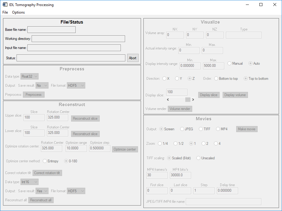
_images/tomo_display_start.png — **tomo_display window on startup**

Note that all regions of the screen are disabled.

Read camera file

To begin process use the File/Read camera file menu to browse for a raw data file. This can be a single .h5 for recent data, or any of the 3 .nc files for pre-2020 dataset. After reading the file the screen will look like this:

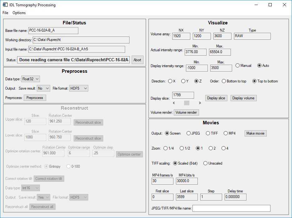
_images/tomo_display_after_read_camera.png — **tomo_display window after reading a camera file**

Note the the Preprocess, Visualize, and Movies screen regions are now enabled.

Visualizing raw data

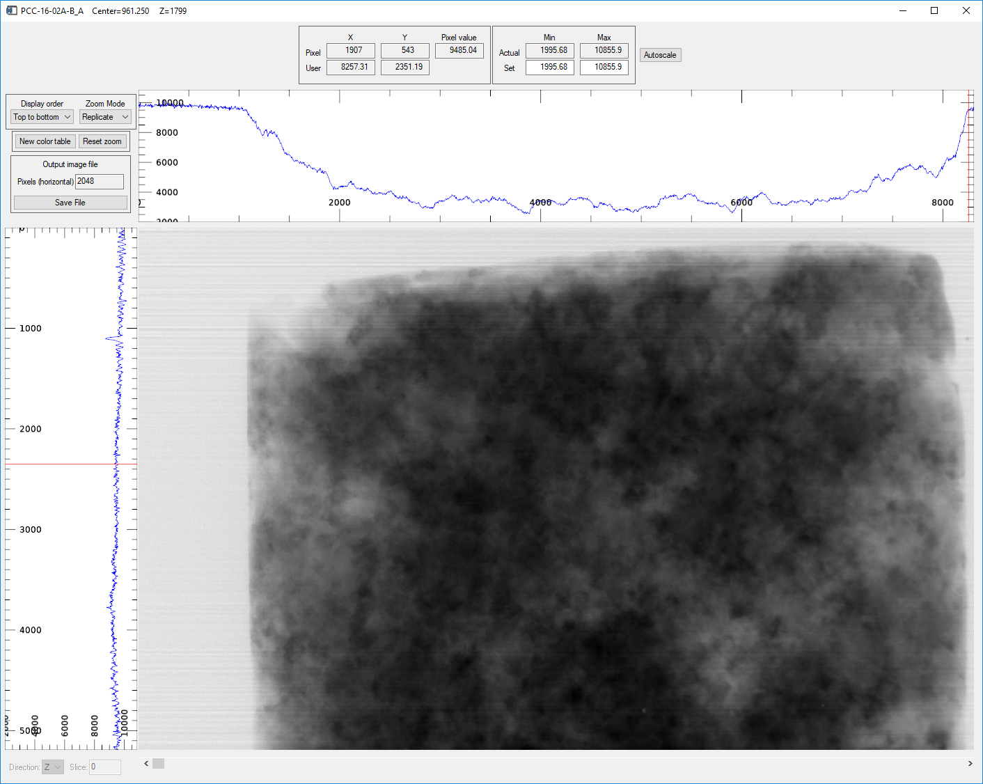
Pressing the Display slice button in the Visualize region opens an image_display window like this:

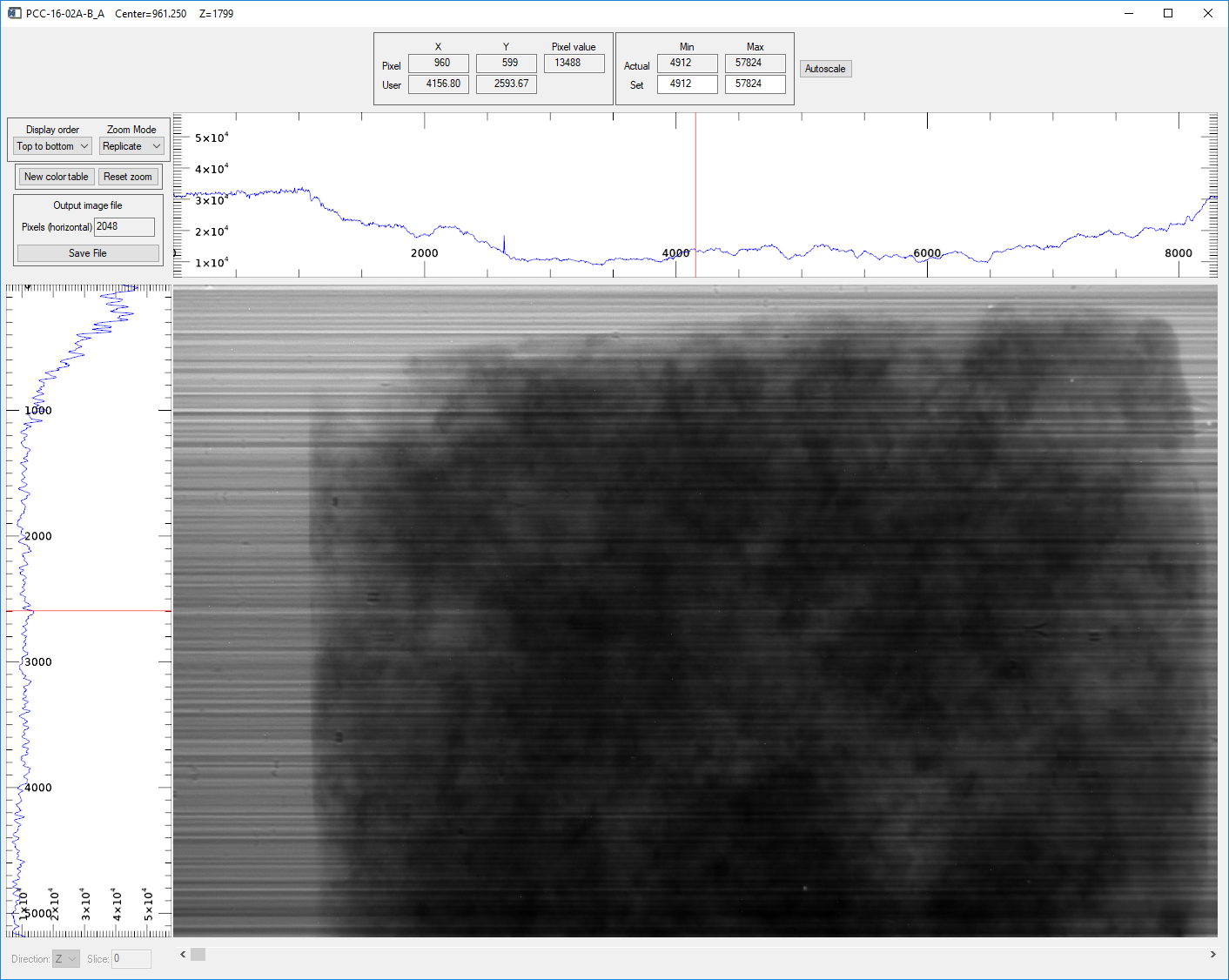
_images/image_display_raw_Z.png — **image_display window showing the raw camera data in the Z direction (projection)**

Preprocessing

Pressing the Preprocess button in the Preprocess region will perform preprocessing. This consists of

Subtracting the dark current from all flat fields and projections
Averaging the flat fields and removing zingers (hot pixels) from them using double-correlation
Dividing each projection by the average flat field, and multiplying by a scale factor (default=10000)
Removing zingers from the normalized projections
If the Data type is UInt16 converts to that data type. Float32 should normally be used if not saving to disk.
Optionally saving the normalized data to an HDF5 or netCDF file

After preprocessing the screen will look like this:

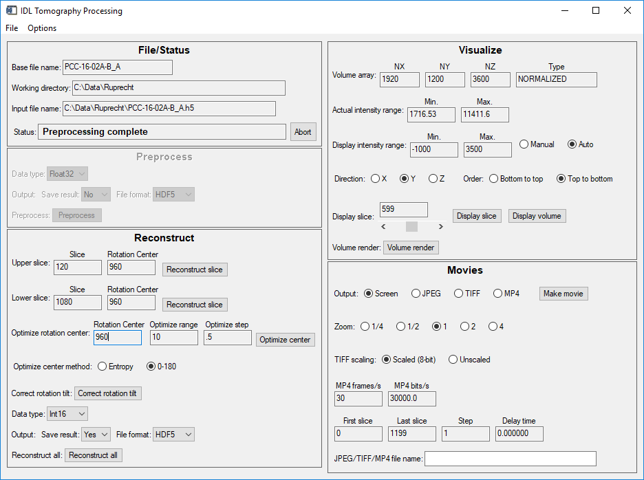
_images/tomo_display_after_preprocess.png — **tomo_display window after preprocessing**

Visualizing normalized data

Pressing the Display slice button in the Visualize region with Direction=Z opens an image_display window like this:

_images/image_display_normalized_Z.png — **image_display window showing the normalized projection in the Z direction (projection)**

Pressing the Display slice button in the Visualize region with Direction=Y opens an image_display window like this:

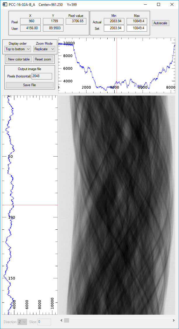
_images/image_display_normalized_Y.png — **image_display window showing the normalized projection in the Y direction (sinogram)**

Optimizing rotation center

Selecting optimization method

There are two methods available for optimizing the rotation center, “Entropy” and “0-180”.

Entropy reconstructs the slices with different rotation centers using the user-specified range and step size. It computes the image entropy for each center, and selects the optimum center as the one with the lowest entropy. Entropy is measured using the sharpness of the image histogram. The entropy technique typically works well for images that are dominated by absorption contrast (rather than phase contrast), and for which the entire sample is mostly in the field of view. It can fail for other types of data. There is in principle no limit to the resolution of the entropy method, and it can easily resolve rotation centers to less than 0.25 pixels.

0-180 is a simpler and faster method. It uses the projections at 0 degrees and 180 degrees. The 180 degree image is reversed in the horizontal direction, and subtracted from the 0 degree image. If the rotation axis were exactly in the middle and the data had no noise or systematic errors then all pixels in the difference should be 0. It then shift the 180 degree image in 1 pixel increments over the user-specified range and step, and determines at which shift the difference is a minimum. 0-180 is more robust than the entropy method, and works even for images dominated by phase contrast or larger than the field of view.

Selecting slices for optimization

The optimization is done for two slices, one near the top of the dataset and one near the bottom. By default these slices are 10% down from the top and 10% up from the bottom. The user may need to adjust these slice numbers to select slices that are in the sample, and not in the air or in very absorbing regions in the top or bottom of the sample. The slice numbers can be selected by using Display slice in the Z direction, moving the cursor and recording the Y pixel value in the desired slices.

Selecting center, range and step for optimization

The Rotation center field selects the center of the range to be used in the optimization. The Optimize range field selects the full range of the optimization, i.e. the optimization range is from center-range/2 to center+range/2. The Rotation step field selects the step size in pixels for the optimization. For the entropy method there is in principle no limit to how small the step size can be, and it can easily resolve rotation centers to less than 0.25 pixels. The 0-180 method has a minimum useful step size of 0.5 pixels, because the shifts are limited to integer pixel increments.

Manual optimization

If neither neither the entropy or 0-180 methods produce satisfactory results, it is possible to manually optimize the center. For both the upper and lower slices manually change the Rotation center for that slice and press Reconstruct slice. Determine which rotation center gives a reconstruction with the fewest artifacts. Slices with small highly absorbing objects are ideal for this, since they show “crescents” facing left or right if the center is wrong. The centers in the upper and lower slices should be very similar.

Correcting rotation tilt

The reason for using slices near the top and bottom is to judge whether the rotation axis is correctly aligned to be parallel to the columns in the camera. If it is then the center will be the same at the top and bottom. If it is not, and the error is significant (e.g. 1 pixel or more) there are two ways to fix the problem. The first is to use the Correct rotation tilt button. This will rotate all of the projections by the angular error, and hence make the rotation center be the same on the top and bottom. The second method is to adjust the mechanical alignment of the system for future datasets.

Optimization plots

This is the plot produced when optimizing with the 0-180 method, using center=960, range=10, step=0.5 It found the optimum center of 961.5 for the upper slice (120) and 961.0 for the lower slice (1080).

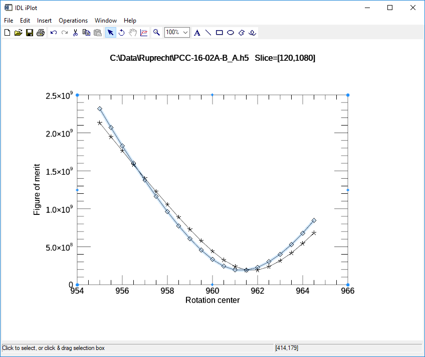
_images/0-180_optimization.png — **0-180 optimization plot**

This is the plot produced when optimizing with the entropy method, using center=960, range=10, step=0.25 It found the optimum center of 961.25 for the upper slice (120) and 960.75 for the lower slice (1080). These values are within 0.25 pixels of those found with the 0-180 method.

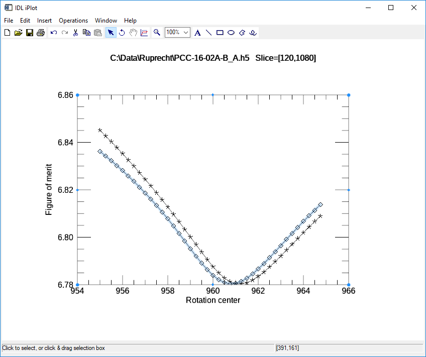
_images/entropy_optimization.png — **Entropy optimization plot**

Reconstruction

Once the optimum rotation center is found, use the Reconstruct all button to reconstruct all of the slices. The output data type can be signed 16-bit integer (Int16), unsigned 16-bit integer (UInt16), or 32-bit floating point (Float32). Normally Save result is set to Yes, so that the reconstruction is written to a file. It can be set to “No” for tests where only in-memory reconstruction is needed. The output File format can be netCDF or HDF5. HDF5 is faster, more widely used, and recommended. netCDF can be used for backwards compatibility for older datasets.

After reconstruction the screen will look like this. Note that Visualize/Type is now “RECONSTRUCTED”, and the Preprocess and Reconstruct regions are disabled.

_images/tomo_display_after_reconstruction.png — **tomo_display window after reconstruction**

The Actual intensity range shows the min and max values of the reconstructed data. The “Display intensity range” min and max values can be set to control the displayed contrast when Manual is selected.

Pressing the Display slice button in the Visualize region with Direction=Z displays a horizontal slice in an image_display window like this.

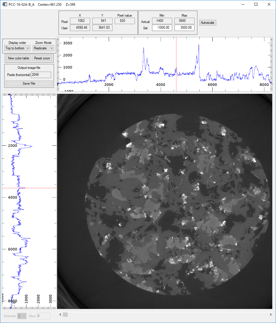
_images/image_display_reconstructed_Z.png — **image_display window showing the center reconstructed slice in the Z (vertical) direction**

Pressing the Display slice button in the Visualize region with Direction=Y displays a vertical slice parallel to the X-ray beam in an image_display window like this.

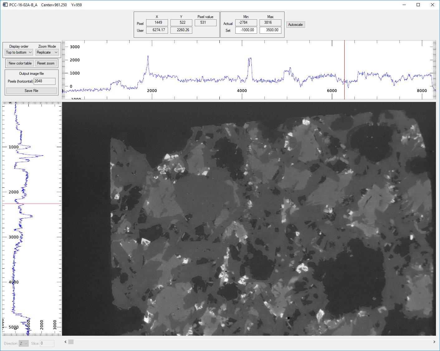
_images/image_display_reconstructed_Y.png — **image_display window showing the center reconstructed slice in the Y direction**

Pressing the Display slice button in the Visualize region with Direction=X displays a vertical slice perpendicular to the X-ray beam in an image_display window like this.

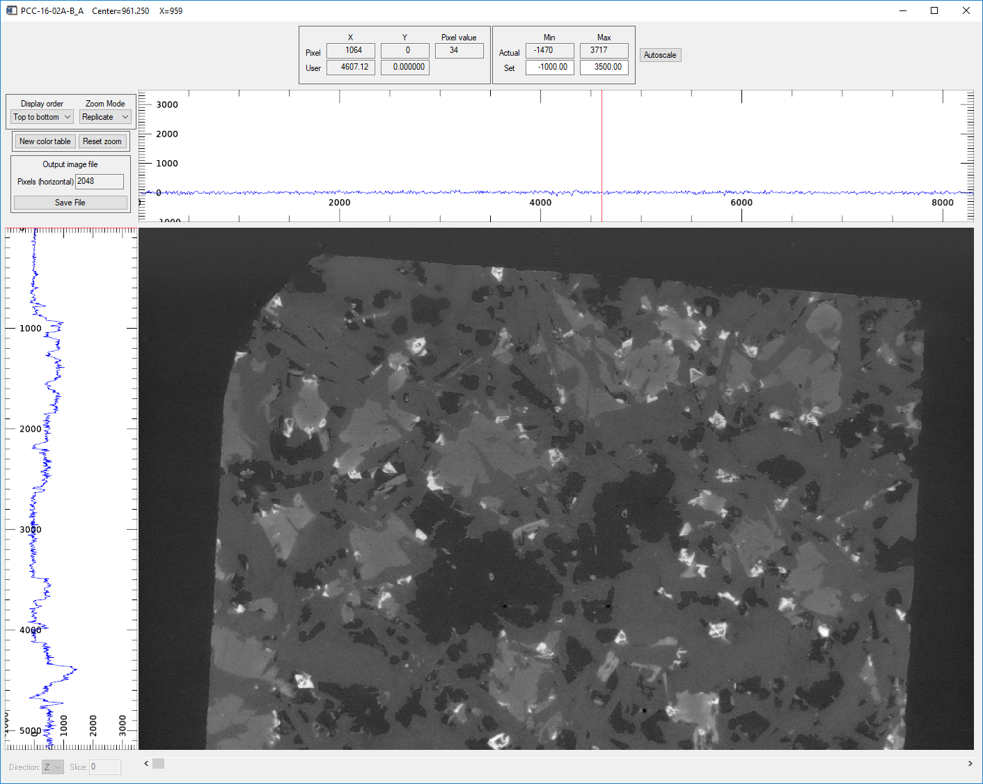
_images/image_display_reconstructed_X.png — **image_display window showing the center reconstructed slice in the X direction**