Processing options
There are a number of options available to control the preprocessing, sinogram, and reconstruction steps. These can be controlled with the Processing Options screen, which is opened with Options/Processing options … in the main tomo_display screen.
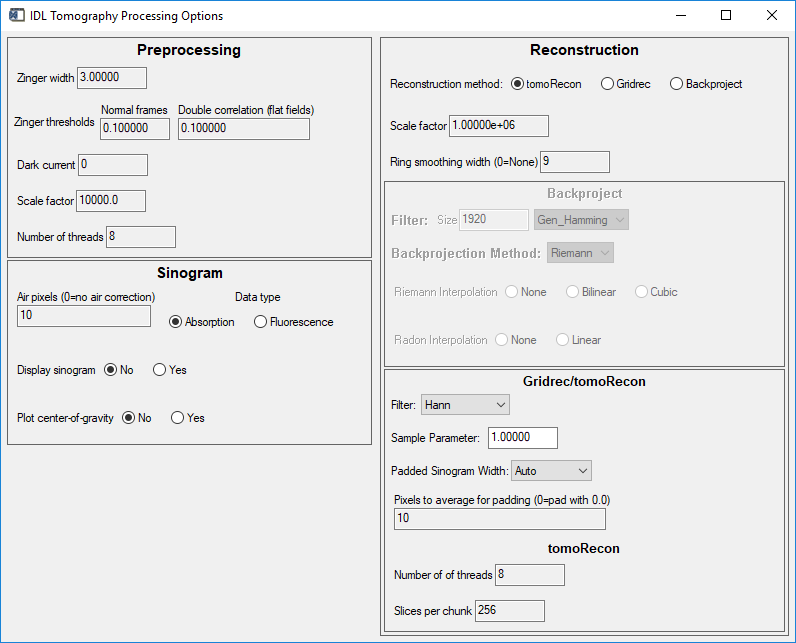
Processing options screen
Preprocessing options
Zinger removal
Zingers are anomalously bright pixels, typically caused by an X-ray directly striking the camera sensor. If they are not removed they will cause single-pixel line artifacts across the image during reconstruction. Zinger removal uses a median-filter algorithm for normal projections, and a double-correlation algorithm for the flat fields. The median filter algorithm has two adjustable parameters:
Zinger width |
This controls the width and height of the median filter window in pixels. |
Zinger threshold |
This is the fractional amount larger than the median value at which a pixel is flagged as a zinger. |
The median filter algorithm does the following:
Computes the median value in a window of size [Zinger width, Zinger width], starting at pixel [0, 0].
Computes the ratio of each pixel value in the window to the median value.
If the ratio is greater than 1 + Zinger threshold then the pixel value is replaced by the median value.
The window is translated horizontally by Zinger width across each row until all columns in that row have been filtered.
The window is translated vertically by Zinger width until all rows have been filtered.
The process is much faster than doing a normal median filter on the entire image. This is because a normal median filter computes the median centered on every pixel in the image, or NX * NY times, where NX and NY are the number of X and Y pixels in the image. The above algorithm only computes the median (NX * NY)/(Zinger width * Zinger width) times. This is 9 times fewer median calculations if Zinger width is 3.
The median filter calculation is done in the multithreaded C++ preprocessing code that also does dark current and flat field correction.
The double correlation algorithm used for flat fields does the following:
Computes the ratio of flat field N and flat field N+1, i.e. N/(N+1)
Computes the median value of the ratio
Divides the ratio by the median value, so the ratio will have an average value near 1.
All pixels in the ratio with values greater than 1 + Zinger threshold are identified as zingers in flat field N.
All pixels in the ratio with values less than 1 - Zinger threshold are identified as zingers in flat field N+1.
The zinger values are replaced by the value of that pixel in the other flat field, scaled by the median ratio.
The double-correlation calculation is done in IDL, which is fast enough for the limited number of flat fields.
Dark current
This value is currently read-only. It is read from the .h5 or .setup files and displayed in this screen for information. The option to allow changing the value in this screen could be added in the future if needed.
Scale factor (preprocessing)
During the preprocessing each projection is divided by the average of the flat fields. This produces a normalized image whose intensity if approximately in the range of 0.0 to 1.0. If one wants to have the option to save the preprocessed data as an unsigned 16-bit integer then it needs to first be scaled by a scale factor. 10000 is the default scale factor, which will produce normalized values in the approximate range of 0 to 10000. This is more than enough precision for the tomography cameras, which are typically 12-bits. A scale factor of 16000 would handle 16-bit cameras with little danger of overflow (>32K), which would only happen if some pixels were more than 2.0 times brighter than the flat field.
Number of threads
This is the number of threads to use for the C++ preprocessing. It is reasonable to use the number cores in the processing machine. A smaller number could be used if other compute-intensive tasks are to run at the same time.
Sinogram options
Air pixels
The preprocessing does a first stage of normalization by dividing each projection by the average of the flat fields. If Air pixels is greater than 0 then it does the following secondary stage of normalization for each row in the sinogram:
Averages the first Air pixels on the left edge of the row and on the right edge of the row.
Draws a straight line between the left and right average air values.
That line is defined as the actual flat field value, and each pixel is renormalized to the value in that line.
This secondary correction can correct for changes in the overall beam intensity, for example due to drops in storage ring beam current during the measurement.
It can also correct for changes due to drift in the mirror or monochromator optics, providing that the changes are uniform in the horizontal direction. That is often the case for mirror and monochromator drifts.
If Air pixels is 0 then there is no secondary normalization.
Data type
The choices are Absorption and Fluorescence. For Absorption data the logarithm of the normalized data must be computed before reconstruction. For Fluorscence data the logarithm operation is not performed.
Display sinogram
Selecting this option will display the sinogram after the logarithm is performed. This option should only be used when reconstructing single slices, and it can only be used if the reconstruction method is Gridrec or Backproject. With tomoRecon the sinogram is computed in C++, and IDL does not have access to the sinogram.
[Need to put image here once Gridrec and Backproject are working again]
Plot center-of-gravity
Selecting this option will plot the center of gravity of the each row of the sinogram as a function of angle. This can be useful for seeing artifacts like sample motion. It has the same restrictions as displaying the sinogram, i.e. only for single slice reconstructions, and not when using tomoRecon.
[Need to put image here once Gridrec and Backproject are working again]
Reconstruction options
Reconstruction method
tomoRecon |
This uses the Gridrec algorithm running with multiple threads. Each thread performs the sinogram calculation, air normalization, ring artifact reduction, and reconstruction for two slices at a time. It is by far the fastest method, and is the default. |
Gridrec |
This performs the sinogram calculation, air normalization, and ring artifact reduction in IDL. The Gridrec reconstruction is done using the Gridrec algorithm in C code in a single thread. It has the advantage of being able to examine the sinogram and center-of-gravity for diagnostics. It is slower than tomoRecon but faster than Backproject. |
Backproject |
This performs the sinogram calculation, air normalization, and ring artifact reduction in IDL. Reconstruction is done using the IDL radon() function. It has the advantage of being able to examine the sinogram and center-of-gravity for diagnostics. It is the slowest method. |
Scale factor (reconstruction)
The data from the tomography reconstruction is the linear X-ray attenuation coefficient in units of inverse pixel size. They represent the fraction of X-rays absorbed as the beam traverses that single pixel. Since the beam is typically absorbed by 10% to 90% as it traverses ~2K pixels, the absorption in each pixel is quite small, typically in the range of .0001 to .01. If it is desired to save the reconstructed values as signed or unsigned 16-bit integers, rather than floating point values, it is necessary to scale the reconstruction values by a Scale factor.
The default scale factor is 1,000,000 (10^6), which will convert a typical voxel value of .001 to 1000. 1000 can be converted to a 16-bit integer with no significant loss of information, because the noise is always larger than 10^-6.
The scale factor can be set to 1 for no scaling. The reconstructed data would then need to be saved as 32-bit float.
Ring smoothing width
The ring artifact reduction method assumes that the average row of the sinogram should be quite “smooth”, without many high-frequency features. It detects high-frequency anomalies and removes them.
If Ring smoothing width is non-zero then ring artifact reduction is performed using the following algorithm before reconstruction for each slice.
The average row of the sinogram is computed.
The smoothed average row is computed using a boxcar filter of width Ring smoothing width.
The difference row (average row minus average smoothed row) is computed.
That difference row is subtracted from each row in the sinogram.
The default Ring smoothing width is 9, which quite effectively removes narrow ring artifacts. By using larger values for Ring smoothing width wider ring artifacts can be removed. However, very large values can introduce new artifacts, and this depends on the structures in the sample. Setting the value to 0 will prevent any ring artifact correction from being performed.
One common problem is a sample in a cylindrical container which is close to being centered on the rotation axis. The inner and outer edges of the cylinder wall will be detected as ring artifacts, and the algorithm can cause new features because of this.
Backproject
The following parameters are available when the reconstruction method is Backproject.
Filter size |
The number of pixels in the filter used before backprojection. |
Filter type |
The type of filter to use. Choices are Gen_Hamming, Shepp_Logan, LP_Cosine, Ramlak, and None. |
Backprojection method |
Choices are Riemann and Radon. |
Riemann interpolation |
The intepolation method to use with Riemann backprojection. Choices are None, Bilinear, and Cubic. |
Radon interpolation |
The intepolation method to use with Radon backprojection. Choices are None and Linear. |
Gridrec/tomoRecon
The following parameters are available when the reconstruction method is either Gridrec or tomoRecon.
Filter |
The filter to use with reconstruction. Choices are Shepp-Logan, Hann, Hamming, and Ramlak. |
Sample parameter |
The sample parameter in the Gridrec algorithm. We need an explanation of what this does. |
Padded sinogram width |
The width to which to pad the sinogram. Choices are Auto, No Padding, 1024, 2048, and 4096. Auto selects the next power of 2 that is >= the width of the projections. Reconstructions are more accurate with larger padding, as the expense of computing time. |
Pixel to average for padding |
When the sinogram is padded this selects the number of pixels from the right and left edges to average when computing the padding value. 0 selects a padding value of 0. |
tomoRecon
The following parameters are available when the reconstruction method is tomoRecon.
Number of threads |
This is the number of threads to use for the C++ reconstruction. It is reasonable to use the number cores in the processing machine. A smaller number could be used if other compute-intensive tasks are to run at the same time. |
Slices per chunk |
The reconstruction can be done in chunks to reduce the amount of memory required. This is the number of slices in each chunk. Not currently implemented. |
NOTE: Chunking was implemented in R1-0 of tomo_display. It is not currently implemented because that requires writing the output files in chunks, and that is not currently supported in the tomo class for HDF5 files.
For detectors with 3K x 3K pixels the reconstructed datasets as 16-bit integers will be 58 GB. he normalized data will be a similar size. Both datasets can thus be memory resident in a machine with 128 GB of RAM. That much memory only costs about $400 today, so chunking is probably not needed until datasets are much larger than this.